portfolio / Metaheuristic Hyperparameter Optimisation _
For my Computational Intelligence module, we applied evolutionary and metaheuristic optimisation to a fine-tuning problem. The goal was to search for the best hyperparameters for LoRA-adapted DistilBERT on an emotion text classification task. It was a group project of four, and my main contributions were implementing the SHADE algorithm from a research paper and working on the multi-objective extension alongside a teammate.
Background
LoRA (Low-Rank Adaptation) is a parameter-efficient fine-tuning method for large pretrained models. Rather than updating all the weights in a model during fine-tuning, it injects small trainable rank decomposition matrices into certain layers and freezes everything else. This ends up reducing the number of trainable parameters and makes fine-tuning feasible on consumer-grade hardware.
LoRA’s own hyperparameters — rank r, scaling factor alpha, dropout, learning rate, warmup ratio, and which layers to target — have a noticeable impact on the final model performance. Choosing them well may not be easy, and brute-force grid search doesn’t scale well as the number of hyperparameters grows. This is where metaheuristic optimisation comes in.
The dataset used was the Emotion dataset, 6 classes of tweets expressing different emotions. We fine-tuned distilbert-base-uncased with a classification head on top, training for 3 epochs per candidate configuration and using validation accuracy as the fitness measure.
The Optimisation Setup
The search space was a mix of continuous and discrete values:
- Learning rate — continuous in
[1e-5, 2e-4] - LoRA rank
r— one of{2, 4, 8, 16, 24} - LoRA alpha — one of
{8, 16, 32, 64, 96} - Warmup ratio — one of
{0.0, 0.06, 0.1} - Dropout — one of
{0.0, 0.05, 0.1, 0.2} - Target modules — attention only, or attention + feedforward
To handle discrete parameters, we used index-based encoding. Each discrete hyperparameter is encoded as an integer index into its list of valid options rather than the value itself. If you’re mutating a rank gene and your valid ranks are {2, 4, 8, 16, 24}, a step-size of 5 in value-space means something very different at rank 4 vs rank 24. Index encoding gives uniform exploration across the options regardless of their spacing.
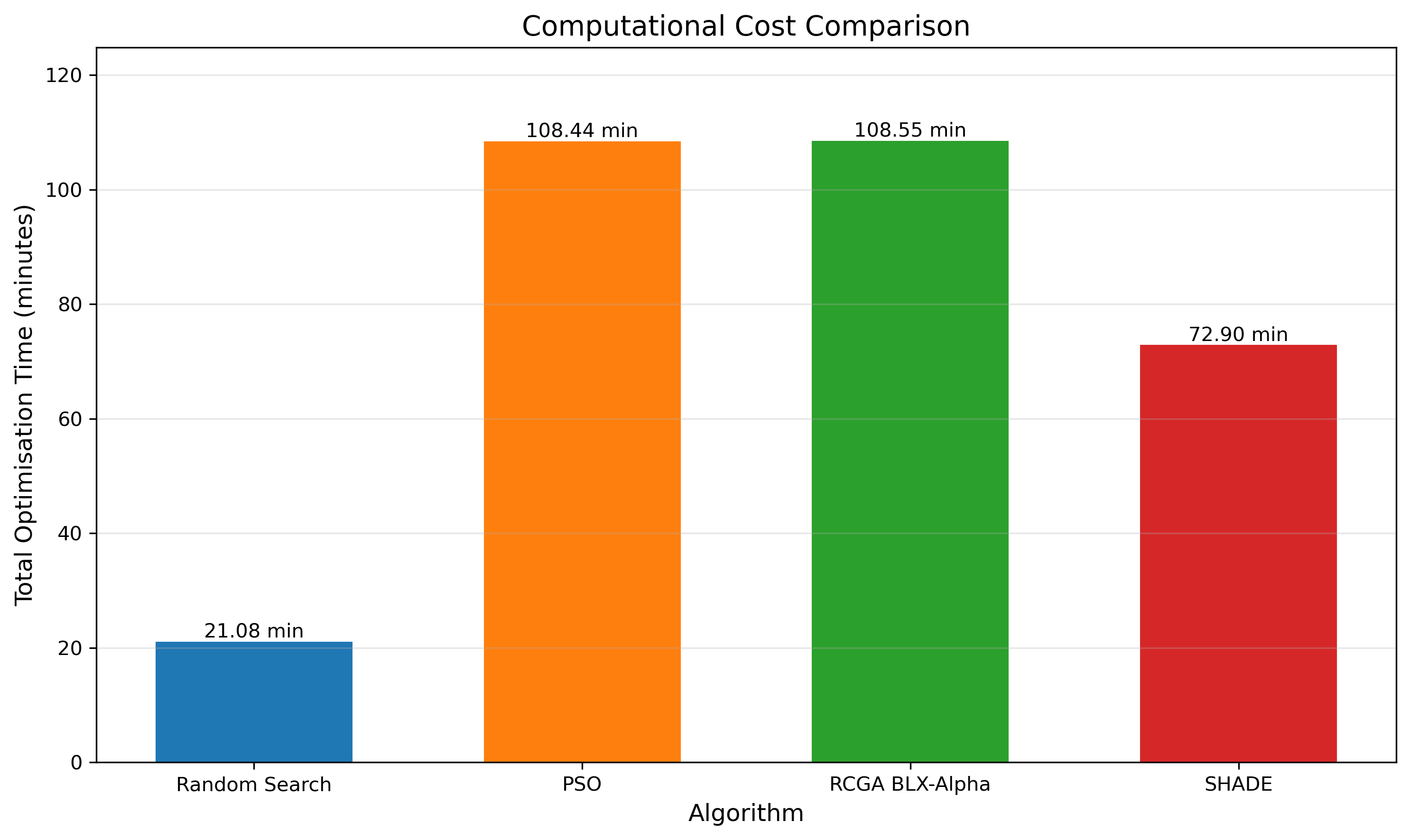
Each candidate configuration required rebuilding the LoRA-wrapped model from scratch, training for 3 epochs, and evaluating on the full validation split. One evaluation took roughly 3–5 minutes on a P100 GPU, which made the total budget very constrained — 100 evaluations for each metaheuristic method (population of 20, 5 generations), and 20 for the random search baseline.
The Algorithms
The coursework asked for four methods: a random search baseline, one population-based heuristic from the module content, and two of our own choice. The group settled on PSO for the population method, and chose RCGA BLX-α and SHADE as the two custom algorithms. I was responsible for modifying SHADE with index-based encoding.
SHADE
SHADE (Success-History based Adaptive Differential Evolution) was the algorithm I researched and implemented. It’s an enhanced variant of Differential Evolution, which wasn’t part of the course content, so it required a bit of digging into the literature.
Standard DE’s main weakness is that you have to manually tune its control parameters. Both crossover rate CR and scaling factor F. The optimal values of these can vary depending on the problem and changing these control parameters affect the convergence rate. SHADE fixes this by maintaining a rolling history of successful CR and F values from previous generations. SHADE samples from that history to adapt the parameters automatically as the search progresses.
Given the limited budget (100 evaluations, 5 generations), the SHADE settings were tuned accordingly. History size, archive rate, p (top % individuals) were chosen to push exploration given the small population.
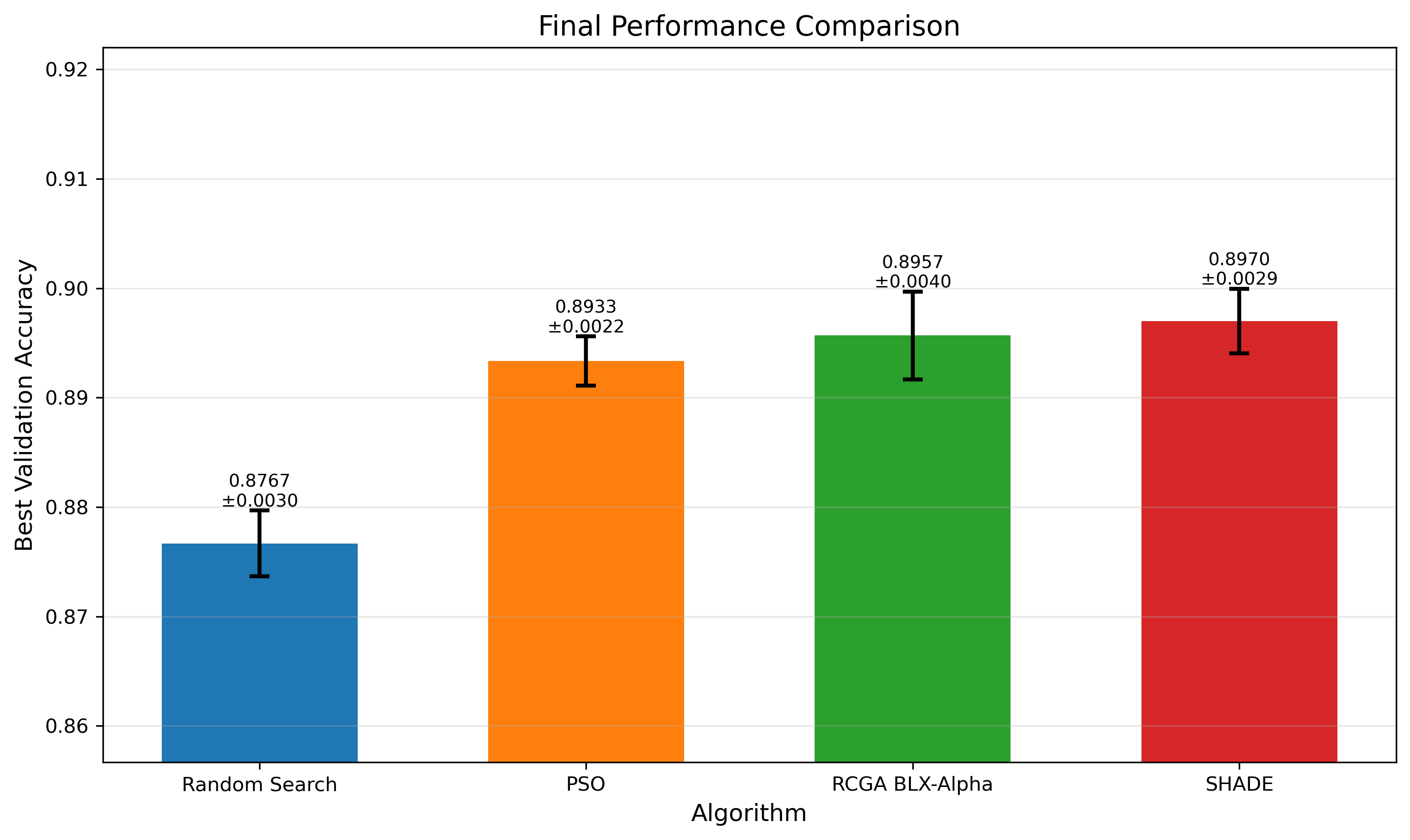
Results
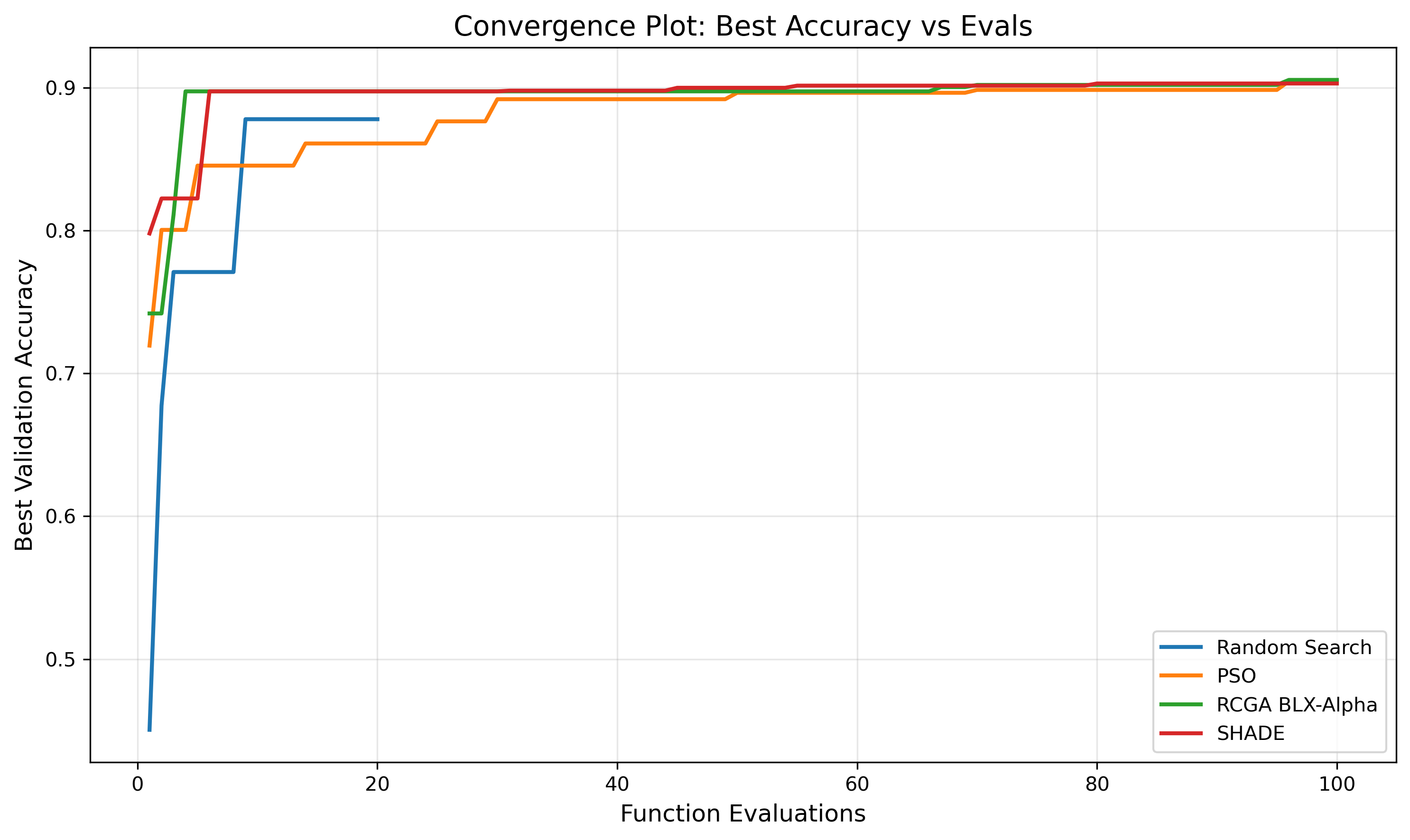
All four algorithms converged to a learning rate of 2×10⁻⁴ and attention+feedforward as the target modules, suggesting these represent strong optima in this search space. The metaheuristic methods also all settled on alpha = 96 and dropout = 0.0, while random search ended up at alpha = 64 and dropout = 0.1 — likely due to its smaller evaluation budget.
| Algorithm | Best Acc. | Mean Acc. | ±Std. | Time (min) |
|---|---|---|---|---|
| Random Search | 0.878 | 0.877 | 0.003 | 21.04 |
| PSO | 0.905 | 0.893 | 0.002 | 108.44 |
| RCGA BLX-α | 0.906 | 0.896 | 0.004 | 108.55 |
| SHADE | 0.900 | 0.897 | 0.003 | 72.90 |
SHADE also finished notably faster. It achieved comparable accuracy to RCGA BLX-α in about 33% less time, making it the most computationally efficient method overall.
An observation after looking at the convergence curve for both SHADE and RCGA, the best configuration was actually found during the random initialisation phase before any generational updates happened. The subsequent generations refined but didn’t really discover anything new. This was a consequence of the constrained discrete search space with only 4–5 valid values per hyperparameter. Random sampling had a reasonable chance of hitting good configurations by chance. In a larger continuous search space, it’s likely that the metaheuristics would pull further ahead.
Multi-Objective Extension
The single-objective algorithms optimise purely for accuracy and ignore model complexity. Two configurations might achieve 85.0% and 85.1% accuracy respectively, but if the latter requires 3× more trainable parameters than the former, a single-objective algorithm simply picks the 85.1% one without question. This is where NSGA-II comes in.
NSGA-II is a multi-objective evolutionary algorithm that doesn’t produce a single best solution, but instead a Pareto front — a set of non-dominated trade-off points. In our case, the two objectives were validation accuracy (to maximise) and number of trainable parameters (to minimise).
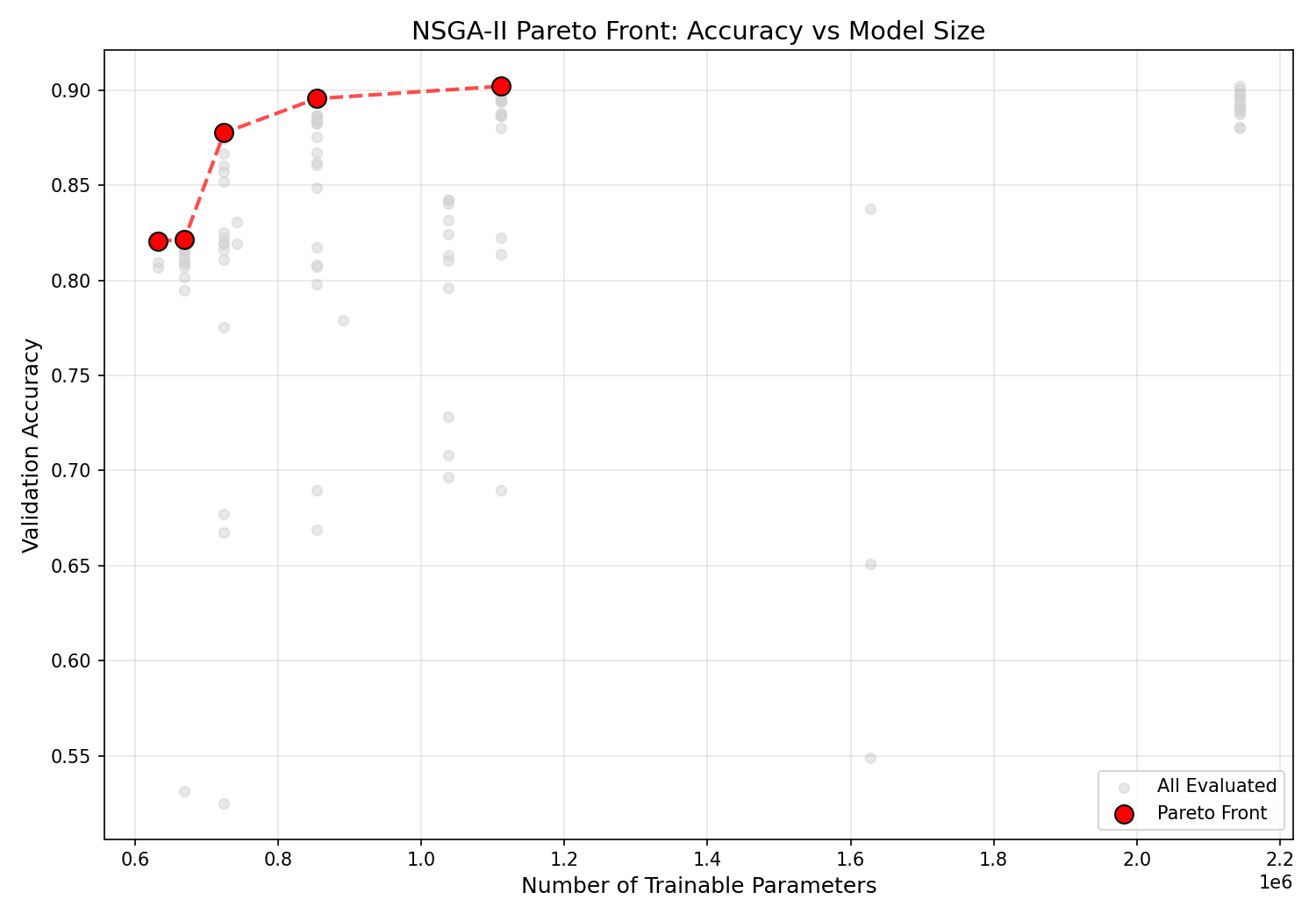
The Pareto front from our run revealed a clear structure. The lowest-parameter solutions (attention-only targets, rank 2–4) sat around 82% accuracy — these configurations visibly underfit the task regardless of rank. The most interesting jump in the front was from 0.67M to 0.72M trainable parameters: a 7.5% increase in parameters that translated to a 5.6% accuracy gain. That step corresponds to switching from attention-only to attention+feedforward targeting, suggesting that adapting the feedforward layers is important for this dataset specifically.
After roughly 0.72M parameters the curve starts to plateau — the last step from 1.11M parameters to the end of the front yielded diminishing returns. So the knee point at around 0.72M is arguably the most efficient configuration in the space.
The multi-objective framing adds something useful here that single-objective optimisation just can’t surface. It makes explicit the question of whether an accuracy gain is worth the added parameter cost — which is a real consideration if you’re constrained by hardware or deployment requirements.
Takeaways
The main thing this project made concrete for me is how much the search space design matters. Because we constrained the discrete options to a small set of values (to keep evaluation costs manageable), the effective dimensionality of the problem was quite low. That’s why random search performed only ~1–2% worse than the best metaheuristic at a fraction of the computational cost. In a setting with a larger search space, you’d expect a larger gap.
SHADE as an algorithm was interesting to implement because the adaptive parameter mechanism means it’s largely self-tuning once you set the history and archive sizes. The core idea of learning from successful past parameter choices rather than requiring manual CR and F tuning was quite elegant.
The multi-objective extension was also interesting. The change of framing from “what’s the best configuration” to “what’s the best configuration given a cost constraint” tends to be more important and used in practice.