portfolio / Dissertation - Regime Targeted Permutation _

After having accumulated experience in algorithmic trading, I decided the best path to take for my dissertation would be financial. After a few iterative improvements of project ideas in supervisor meetings, my project was about researching whether deliberately disrupting specific regions of training data could make a machine learning model more profitable when predicting Bitcoin price movements.

The following will be a summarisation of my dissertation. I thought about adding the full processes including mistakes that were made and lessons learnt, but that would likely double this page length so I omitted them here.

The Problem

Machine learning models trained on historical financial data have a tendency to overfit. The patterns they learn from the training period don’t reliably carry over into the future. This is partly because financial data is non-stationary, meaning that their statistical properties (mostly concerning returns) shift over time. Another reason is because the signal-to-noise ratio in price data is exceptionally low. There’s a lot of noise and very little actual signal.

Most attempts to improve trading strategies (using machine/deep learning) focus on the model side of things: better architectures, more careful hyperparameter tuning, regularisation. What gets less attention is the training data itself.

Data augmentation is standard practice in domains like computer vision, where you can flip, crop, or rotate images to expose a model to more variation. Applying the same idea to financial time series is harder because the statistical properties of return data matter. If you add noise or stretch the time axis you risk distorting the distribution of returns, and the model ends up training on data that doesn’t reflect the real thing.

The central question of my project was: can you permute specific regions of training data in a way that preserves the return distribution but reduces overfitting?

Data

Hourly OHLCV data for BTC-USDT from Binance, January 2018 to January 2026. About 70,000 bars in total, split 70/30 chronologically into training and validation sets.

Cryptocurrency was a deliberate choice. Equity markets close overnight, on weekends, and on public holidays. That creates gaps in the price series, which complicates the permutation method used in this project. Bitcoin trades continuously, so every bar in the dataset is consistent with every other bar. There are no gaps to worry about.

Features

23 features were constructed from the raw price data, grouped into five categories:

• Trend — multi-period log returns, the Kaufman Efficiency Ratio, and the distance of price from its Kaufman Adaptive Moving Average (KAMA)
• Volatility — Average True Range (ATR) at multiple lookbacks, and Bollinger Band width
• Momentum — RSI at multiple periods, normalised close position within the bar, and log high-low range
• Volume — Force Index, z-scored On-Balance Volume, and normalised volume
• Time — hour of day and day of week, encoded as sine and cosine pairs All features were constructed around near-stationarity. XGBoost can’t extrapolate beyond its training range, so features that drift over time — like raw price or cumulative volume — cause the model to degrade during evaluation when values fall outside anything it saw during training. Log-differencing and normalisation deal with most of this.

The target variable was the 3-hour log return.

The Model

An XGBoost regressor. The main reason for this choice was computational efficiency. Since the model needs to be retrained tens of thousands of times across the experiment, anything slow was out. XGBoost also works well with the kind of engineered tabular features being used here, and it supports SHAP analysis, which was needed later to select which features to build permutation types around.

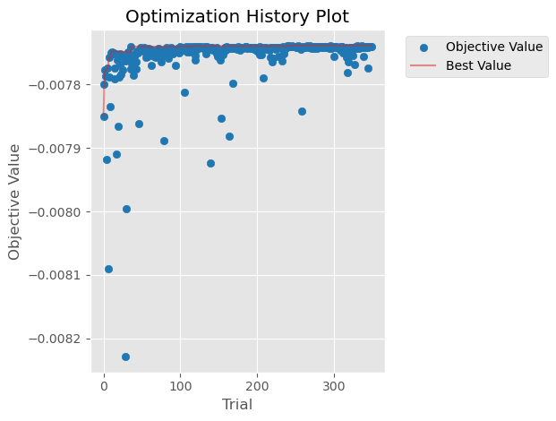
Hyperparameter optimisation was done with Optuna’s TPE sampler over 350 trials, using an expanding-window walk-forward validation scheme across 5 folds. Optimisation was done entirely within the training partition so the validation set was never touched. The selected configuration came out quite conservative. This made sense given how noisy hourly crypto returns are.

The Permutation Function

Before getting to the permutation types, it’s worth explaining what the permutation function actually does.

A naive shuffle of OHLC bars breaks things. If you rearrange bars randomly, you can end up pairing a large intrabar price drop with a large gap upward to the next bar’s open. This is something that essentially never happens in real data.

The approach used here is a bar permutation algorithm developed by Timothy Masters, with a Python port by neurotrader under MIT licence. It solves this by decomposing each bar into two separate series before shuffling:

• The intrabar relatives — the high, low, and close expressed relative to the bar’s open — are shuffled together as locked trios
• The inter-bar gaps — the open-to-prior-close return — are shuffled independently By separating these two series, large intrabar moves can’t accidentally be paired with large inter-bar jumps. The reconstruction chains the permuted components back together bar by bar, working in log-price space throughout.

The key property this preserves is the marginal return distribution: the mean, standard deviation, skew, and kurtosis of the output series are identical to the input. What gets destroyed is the temporal autocorrelation, which is simply the sequential ordering of events. So any observed difference in model performance after permutation has to come from a change in temporal structure alone, not from a shift in what the model is being trained to predict (return data is unchanged).

Permutation Types

A permutation type is a rule for choosing which bars of the training set get passed to the permutation function. Rather than permuting everything uniformly, each type identifies specific contiguous regions of the training data and applies permutation only there. The rest is left unchanged.

Seven types were tested:

Random baselines

• permute_full — permutes the entire training set
• random_50pct — a randomly positioned contiguous 50% block
• random_15pct — a randomly positioned contiguous 15% block Regime-based types — each targeting extreme readings of a SHAP-selected feature, covering approximately 15% of training bars for fair comparison:
• perm_rsi — RSI_50 overbought/oversold extremes (below 39.7 or above 60.3)
• perm_atr — ATR_72 above the 85th percentile (high volatility)
• perm_kama — KAMA distance above a threshold (strong trend)
• perm_fi — Force Index magnitude above a threshold (high volume-driven price force) The features for the regime types were selected via SHAP importance analysis on the tuned model. The rationale being: permuting regions the model ignores produces no meaningful change regardless. Targeting the features the model actually uses makes the permutation relevant.

A minimum of 4 contiguous bars is required for any permutation to occur. The Masters function anchors the first and last bar of any block it receives, leaving only the interior bars free. At 4 bars you get 2 interior bars that can move. So 4 bars is the minimum structural alteration.

Regime Identification

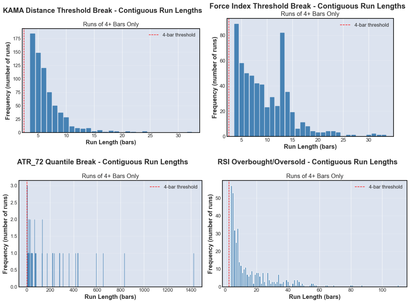
The four regime types ended up looking quite different from each other in terms of their run-length structure.

The RSI, KAMA, and Force Index types all produced many short runs, with medians of 6–9 bars. Only ATR was structurally different: 40 qualifying runs covering 7,339 bars, with a median run length of 69 bars and a single maximum run of 1,423. Where the other types apply frequent small alterations spread across the training set, a single ATR permutation disrupts a small number of very large contiguous segments. This distinction matters for interpreting the results.

The four regimes were also largely non-overlapping at the bar level. 64.2% of training bars were active in zero regimes simultaneously, and only 0.9% were active in all four. The largest pairwise overlap was between KAMA and Force Index at around 52%, which makes sense: strong trending behaviour tends to come with sustained buying or selling pressure, which is exactly what Force Index captures.

Results

Each permutation type was run 5,000 independent times. Each run: permute the training set → recompute all 23 features from scratch on the permuted data → train a fresh model → evaluate on the real, unaltered validation set → record profit factor.

Profit factor is the ratio of gross winning returns to gross losing returns. A value above 1.0 means the strategy is generating more in gross profit than it loses. The real baseline (model trained on unaltered data) came in at 1.1132.

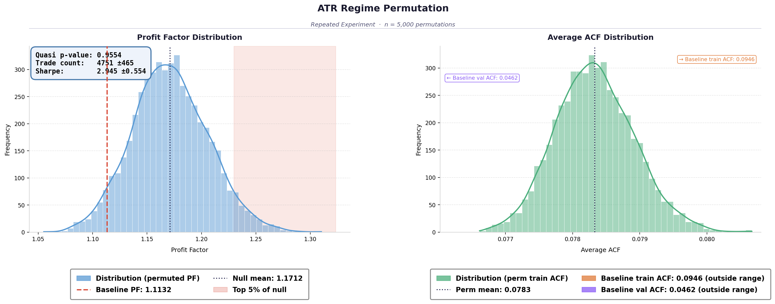
The ATR regime type was the standout result:

• Mean profit factor of 1.1712 across 5,000 runs
• 95.5% of the 5000 individual runs exceeded the real baseline
• Outperformed all three random baselines
• Highest Sharpe ratio of any type tested Force Index produced modest outperformance. RSI and KAMA didn’t improve on the baseline in distributional terms, though RSI showed a weak residual signal that only emerged in the ensemble averaging.

The Interesting Part

The original hypothesis was that permuting regime regions would produce a training set whose structure more closely resembles the validation period — making the model better adapted to what it would encounter when deployed.

That’s not what happened. Or at least, it’s not the right way to describe it.

A structural similarity metric based on autocorrelation was computed on each permuted training series. The idea was to check how close the temporal structure of the permuted data was to the validation set. What became apparent is that permutation is just a destruction operator. Every permutation type moves the training data from structured toward noise. There’s no sense in which you can move a series “closer” to the validation set using permutation — you’re just reducing the autocorrelation structure at different rates. This applies to any replacement metric you could think of: DTW-based, recurrence-based, it doesn’t matter. They all track the same axis.

So the ATR result needs a different explanation, and the better one is this: permuting the high-volatility training periods prevents the model from overfitting to patterns that only exist in those periods. The improvement is about what gets removed, not what gets produced.

This was confirmed with an additional inverse ATR experiment. Instead of permuting the top 15% of bars by volatility, the threshold was flipped so that the bottom 85% was permuted — leaving only the extreme periods intact.

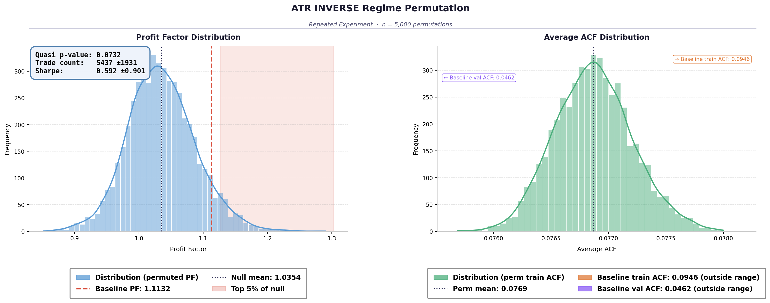
Performance collapsed. The inverse type produced a mean profit factor of 1.0354, the weakest of anything tested. When only the high-volatility periods remain intact as training signal, the model learns nothing useful.

The implication is that the generalisable signal in the training data is concentrated in the ordinary, mild-regime market state. The extreme events — the periods that practitioners tend to focus on most — appear to be actively harmful for generalisation. The model overfits to patterns specific to those periods that don’t carry forward.

As a speculative extension of this: the conventional overbought/oversold thresholds in technical analysis (RSI at 70/30 and similar) might mark regions of elevated noise more than elevated signal. The price behaviour leading up to those extremes could carry more predictive content than the extremes themselves. That’s not something a single experiment on one asset can establish, but it’s a hypothesis the data is consistent with.

Limitations

A few things worth flagging:

• The study uses a single asset (BTC-USDT) and a single model class (XGBoost). Whether the ATR result generalises to other assets or model architectures is untested.
• Equal bar coverage across regime types doesn’t mean equal structural impact. ATR’s very long runs produce much larger price path deviations than the short fragmented runs of RSI, KAMA, or Force Index. It’s not possible to fully disentangle whether the ATR outperformance comes from targeting the right regime or simply from applying more structural disruption per run.
• Coverage calibration was applied before the 4-bar minimum filter, leaving effective bar counts lower than intended and uneven across types.
• No transaction costs were modelled. The profit factor improvements are observed in a frictionless simulation.

Reflection

The most valuable thing this project produced wasn’t the ATR result — it was the inverse ATR experiment and the conclusion that followed from it. A result that contradicts the original hypothesis ends up being more informative than one that confirms it, provided you take it seriously.

The structural similarity metric being effectively useless as a directional measure was also a useful thing to realise, even if it came later than it should have. It clarified what the permutation framework is actually doing and reframed the interpretation of everything else.

The experiment framework — 5,000 independent runs per type producing a distribution of outcomes — is reusable. The questions it leaves open are hopefully as much a contribution as the answers it provides.

The full dissertation is available on request. The code is structured across five Python modules and is reproducible from the raw OHLCV data file and fixed random seeds alone.